Generative Models - Variational Autoencoders
🎙️ Alfredo CanzianiRecap: Auto-encoder (AE)
To summarize at a high level, a very simple form of AE is as follows:
- First, the autoencoder takes in an input and maps it to a hidden state through an affine transformation $\boldsymbol{h} = f(\boldsymbol{W}_h \boldsymbol{x} + \boldsymbol{b}_h)$, where $f$ is an (element-wise) activation function. This is the encoder stage. Note that $\boldsymbol{h}$ is also called the code.
- Next, $\hat{\boldsymbol{x}} = g(\boldsymbol{W}_x \boldsymbol{h} + \boldsymbol{b}_x)$, where $g$ is an activation function. This is the decoder stage.
For a detailed explaination, refer to the notes of Week 7.
Intuition behind VAE and a comparison with classic autoencoders
Next, we introduce Variational Autoencoders (or VAE), a type of generative models. But why do we even care about generative models? To answer the question, discriminative models learn to make predictions given some observations, but generative models aim to simulate the data generation process. One effect is that generative models can better understand the underlying causal relations which leads to better generalization.
Note that although VAE has “Autoencoders” (AE) in its name (because of structural or architectural similarity to auto-encoders), the formulations between VAEs and AEs are very different. See Figure 1 below.
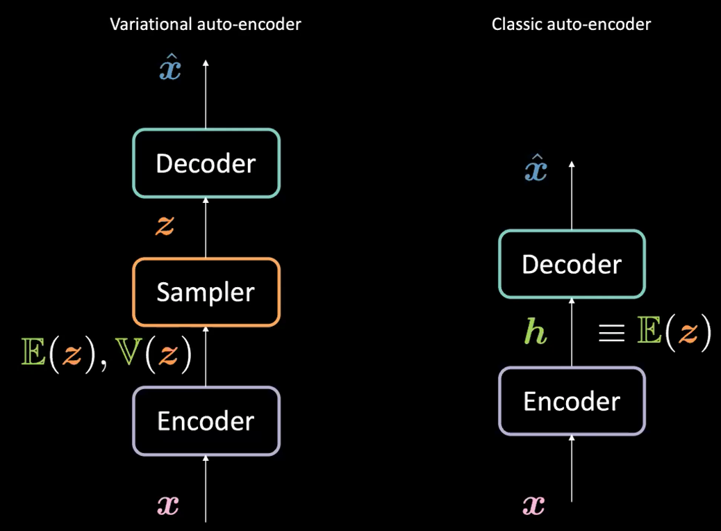
Fig. 1: VAE vs. Classic AE
What’s the difference between variational auto-encoder (VAE) and classic auto-encoder (AE)?
For VAE:
- First, the encoder stage: we pass the input $\boldsymbol{x}$ to the encoder. Instead of generating a hidden representation $\boldsymbol{h}$ (the code) in AE, the code in VAE comprises two things: $\mathbb{E}(\boldsymbol{z})$ and $\mathbb{V}(\boldsymbol{z})$ where $\boldsymbol{z}$ is the latent random variable following a Gaussian distribution with mean $\mathbb{E}(\boldsymbol{z})$ and variance $\mathbb{V}(\boldsymbol{z})$. Note that people use Gaussian distributions as the encoded distribution in practice, but other distributions can be used as well.
- The encoder will be a function from $\mathcal{X}$ to $\mathbb{R}^{2d}$: $\boldsymbol{x} \mapsto \boldsymbol{h}$ (here we use $\boldsymbol{h}$ to represent the concatenation of $\mathbb{E}(\boldsymbol{z})$ and $\mathbb{V}(\boldsymbol{z})$).
- Next, we will sample $\boldsymbol{z}$ from the above distribution parametrized by the encoder; specifically, $\mathbb{E}(\boldsymbol{z})$ and $\mathbb{V}(\boldsymbol{z})$ are passed into a sampler to generate the latent variable $\boldsymbol{z}$.
- Next, $\boldsymbol{z}$ is passed into the decoder to generate $\hat{\boldsymbol{x}}$.
- The decoder will be a function from $\mathcal{Z}$ to $\mathbb{R}^{n}$: $\boldsymbol{z} \mapsto \boldsymbol{\hat{x}}$.
In fact, for classic autoencoder, we can think of $\boldsymbol{h}$ as just the vector $\E(\boldsymbol{z})$ in the VAE formulation. In short, the main difference between VAEs and AEs is that VAEs have a good latent space that enables generative process.
The VAE objective (loss) function
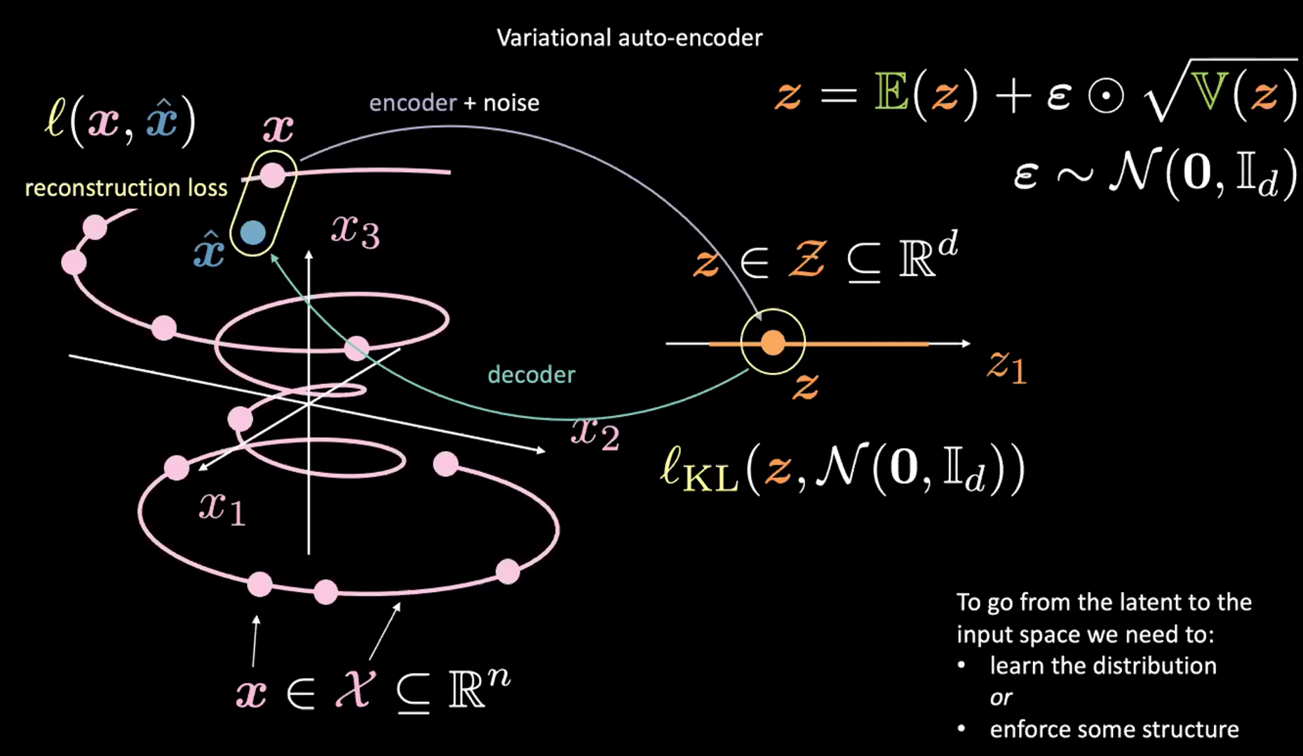
Fig. 2: Mapping from input space to latent space
See Figure 2 above. For now, ignore the top-right corner (which is the reparameterisation trick explained in the next section).
First, we encode from input space (left) to latent space (right), through encoder and noise. Next, we decode from latent space (right) to output space (left). To go from the latent to input space (the generative process) we will need to either learn the distribution (of the latent code) or enforce some structure. In our case, VAE enforces some structure to the latent space.
As usual, to train VAE, we minimize a loss function. The loss function is therefore composed of a reconstruction term as well as a regularization term.
- The reconstruction term is on the final layer (left side of the figure). This corresponds to $l(\boldsymbol{x}, \hat{\boldsymbol{x}})$ in the figure.
- The regularization term is on the latent layer, to enforce some specific Gaussian structure on the latent space (right side of the figure). We do so by using a penalty term $l_{KL}(\boldsymbol{z}, \mathcal{N}(\boldsymbol{0}, \boldsymbol{I}_d))$. Without this term, VAE will act like a classic autoencoder, which may lead to overfitting, and we won’t have the generative properties that we desire.
Discussion on sampling $\boldsymbol{z}$ (reparameterisation trick)
How do we sample from the distribution returned by the encoder in VAE? According to above, we sample from the Gaussian distribution, in order to obtain $\boldsymbol{z}$. However, this is problematic, because when we do gradient descent to train the VAE model, we don’t know how to do backpropagation through the sampling module.
Instead, we use the reparameterization trick to “sample” $\boldsymbol{z}$. We use $\boldsymbol{z} = \mathbb{E}(\boldsymbol{z}) + \boldsymbol{\epsilon} \odot \sqrt{\mathbb{V}(\boldsymbol{z})}$ where $\epsilon\sim \mathcal{N}(\boldsymbol{0}, \boldsymbol{I}_d)$. In this case, backpropagation in training is possible. Specifically, the gradients will go through the (element-wise) multiplication and addition in the above equation.
Breaking apart the VAE Loss Function
Visualizing Latent Variable Estimates and Reconstruction Loss
As stated above, the loss function for the VAE contains two parts: a reconstruction term and a regularization term. We can write this as
\[l(\boldsymbol{x}, \hat{\boldsymbol{x}}) = l_{reconstruction} + \beta l_{\text{KL}}(\boldsymbol{z},\mathcal{N}(\textbf{0}, \boldsymbol{I}_d))\]To visualize the purpose of each term in the loss function, we can think of each estimated $\boldsymbol{z}$ value as a circle in $2d$ space, where the centre of the circle is $\mathbb{E}(\boldsymbol{z})$ and the surrounding area are the possible values of $\boldsymbol{z}$ determined by $\mathbb{V}(\boldsymbol{z}).$
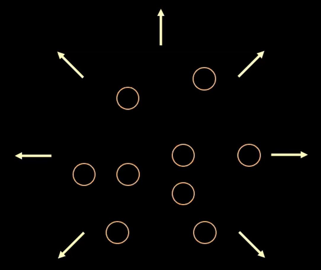
Fig. 3: Visualizing vector $z$ as bubbles in the latent space
In Figure 3 above, each bubble represents an estimated region of $\boldsymbol{z}$, and the arrows represent how the reconstruction term pushes each estimated value away from the others, which is explained more below.
If there is overlap between any two estimates of $z$, (visually, if two bubbles overlap) this creates ambiguity for reconstruction because the points in the overlap can be mapped to both original inputs. Therefore the reconstruction loss will push the points away from one another.
However, if we use just the reconstruction loss, the estimates will continue to be pushed away from each other and the system could blow up. This is where the penalty term comes in.
Note: for binary inputs the reconstruction loss is
\[l(\boldsymbol{x}, \hat{\boldsymbol{x}}) = - \sum\limits_{i=1}^n [x_i \log{(\hat{x_i})} + (1 - x_i)\log{(1-\hat{x_i})}]\]and for real valued inputs the reconstruction loss is
\[l(\boldsymbol{x}, \hat{\boldsymbol{x}}) = \frac{1}{2} \Vert\boldsymbol{x} - \hat{\boldsymbol{x}} \Vert^2\]The penalty term
The second term is the relative entropy (a measure of the distance between two distributions) between $\boldsymbol{z}$ which comes from a Gaussian with mean $\mathbb{E}(\boldsymbol{z})$, variance $\mathbb{V}(\boldsymbol{z})$ and the standard normal distribution. If we expand this second term in the VAE loss function we get:
\[\beta l_{\text{KL}}(\boldsymbol{z},\mathcal{N}(\textbf{0}, \boldsymbol{I}_d)) = \frac{\beta}{2} \sum\limits_{i=1}^d(\mathbb{V}(z_i) - \log{[\mathbb{V}(z_i)]} - 1 + \mathbb{E}(z_i)^2)\]Where each expression in the summation has four terms. Below we write out and graph the first three terms in Figure 4.
\[v_i = \mathbb{V}(z_i) - \log{[\mathbb{V}(z_i)]} - 1\]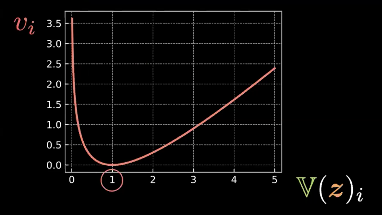
Fig. 4: Plot showing how relative entropy forces the bubbles to have variance = 1
So we can see that this expression is minimized when $z_i$ has variance 1. Therefore our penalty loss will keep the variance of our estimated latent variables at around 1. Visually, this means our “bubbles” from above will have a radius of around 1.
The last term, $\mathbb{E}(z_i)^2$, minimizes the distance between the $z_i$ and therefore prevents the “exploding” encouraged by the reconstruction term.
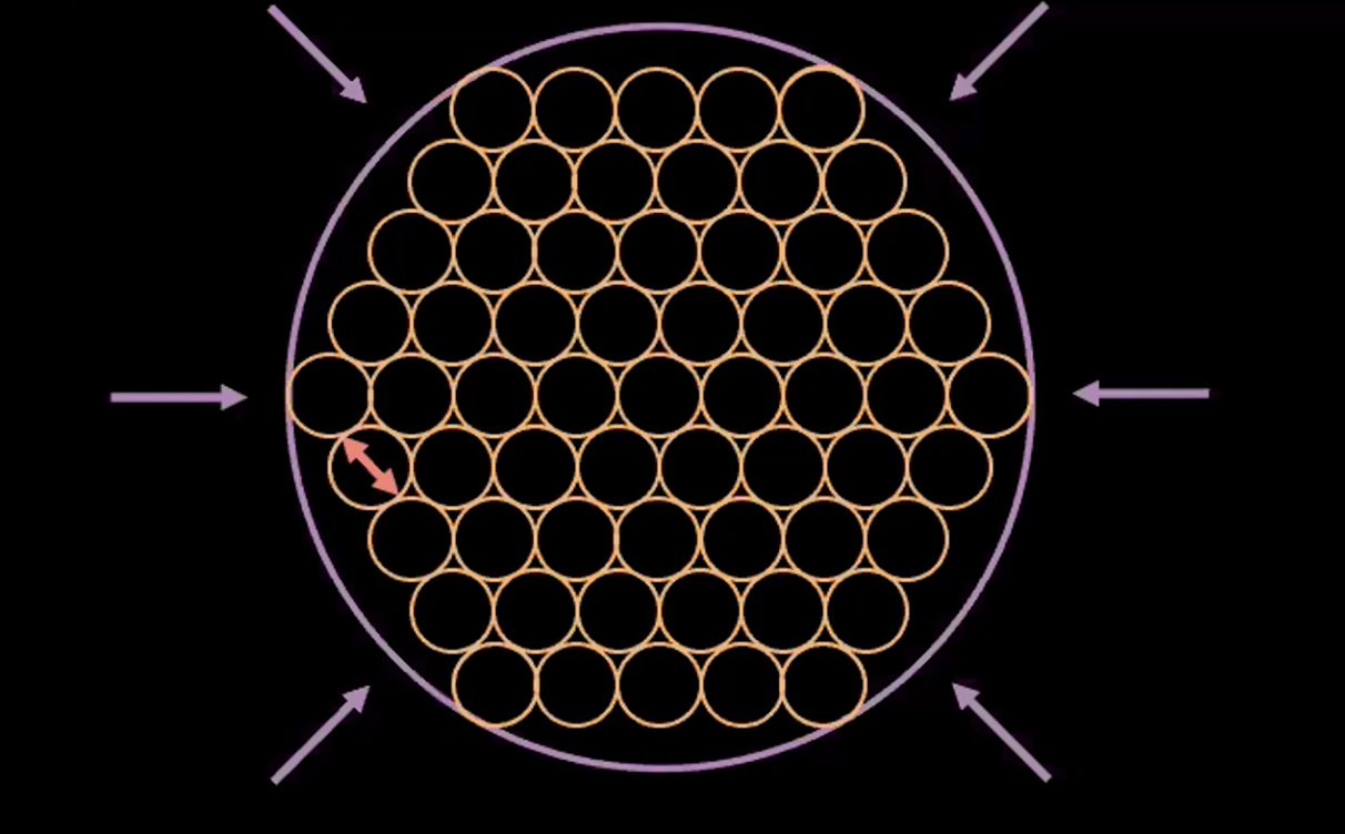
Fig. 5: The "bubble-of-bubble" interpretation of VAE
Figure 5 above shows how VAE loss pushed the estimated latent variables as close together as possible without any overlap while keeping the estimated variance of each point around one.
Note: The $\beta$ in the VAE loss function is a hyperparameter that dictates how to weight the reconstruction and penalty terms.
Implementation of Variational Autoencoder (VAE)
The Jupyter notebook can be found here.
In this notebook, we implement a VAE and train it on the MNIST dataset. Then we sample $\boldsymbol{z}$ from a normal distribution and feed to the decoder and compare the result. Finally, we look at how $\boldsymbol{z}$ changes in 2D projection.
Note: In the MNIST dataset used, the pixel values have been normalized to be in range $[0, 1]$.
The Encoder and the Decoder
- We define the encoder and decoder in our
VAEmodule. - For the last linear layer of encoder, we define the output to be of size $2d$, of which the first $d$ values are the means and the remaining $d$ values are the variances. We sample $\boldsymbol{z} \in R^d$ using these means and variances as explained in the reparameterisation trick before.
- For the last linear layer in the decoder, we use the sigmoid activation so that we can have output in range $[0, 1]$, similar to the input data.
class VAE(nn.Module):
    def __init__(self):
        super().__init__()

        self.encoder = nn.Sequential(
            nn.Linear(784, d ** 2),
            nn.ReLU(),
            nn.Linear(d ** 2, d * 2)
        )

        self.decoder = nn.Sequential(
            nn.Linear(d, d ** 2),
            nn.ReLU(),
            nn.Linear(d ** 2, 784),
            nn.Sigmoid(),
        )
Reparameterisation and the forward function
For the reparameterise function, if the model is in training mode, we compute the standard deviation (std) from log variance (logvar). We use log variance instead of variance because we want to make sure the variance is non-negative, and taking the log of it ensures that we have the full range of the variance, which makes the training more stable.
During training, the reparameterise function will do the reparameterisation trick so that we can do backpropagation in training. To connect to the concept of a yellow bubble, as explained in the lecture, every time this function is called, we draw a point eps = std.data.new(std.size()).normal_(), so if we do 100 times, we will get 100 points which roughly forms a sphere because it’s normal distribution, and the line eps.mul(std).add_(mu) will make this sphere centred in mu with radius equal to std.
For the forward function, we first compute the mu (first half) and logvar (second half) from the encoder, then we compute the $\boldsymbol{z}$ via the reparamterise function. Finally, we return the output of the decoder.
def reparameterise(self, mu, logvar):
    if self.training:
        std = logvar.mul(0.5).exp_()
        eps = std.data.new(std.size()).normal_()
        return eps.mul(std).add_(mu)
    else:
        return mu

def forward(self, x):
    mu_logvar = self.encoder(x.view(-1, 784)).view(-1, 2, d)
    mu = mu_logvar[:, 0, :]
    logvar = mu_logvar[:, 1, :]
    z = self.reparameterise(mu, logvar)
    return self.decoder(z), mu, logvar
Loss function for the VAE
Here we define the reconstruction loss (binary cross entropy) and the relative entropy (KL divergence penalty).
def loss_function(x_hat, x, mu, logvar):
    BCE = nn.functional.binary_cross_entropy(
        x_hat, x.view(-1, 784), reduction='sum'
    )
    KLD = 0.5 * torch.sum(logvar.exp() - logvar - 1 + mu.pow(2))

    return BCE + KLD
Generating new samples
After we train our model, we can sample a random $z$ from the normal distribution and feed it to our decoder. We can observe in Figure 6 that some of the results are not good because our decoder has not “covered” the whole latent space. This can be improved if we train the model for more epochs.

Fig. 6: Randomly moving in the latent space
We can look at how one digit morphs into another, which would not have been possible if we used an autoencoder. We can see that when we walk in the latent space, the output of the decoder still looks legit. Figure 7 below shows how we morph the digit $3$ to $8$.
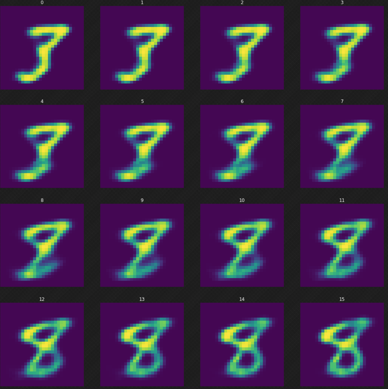
Fig. 7: Morphing the digit 3 into 8
Projection of means
Finally, let’s take a look at how the latent space changes during/after training. The following charts in Figure 8 are the means from the output of the encoder, projected on 2D space, where each colour represents a digit. We can see that from epoch 0, the classes are spreading everywhere, with only little concentration. As the model is trained, the latent space becomes more well-defined and the classes (digits) starts to form clusters.
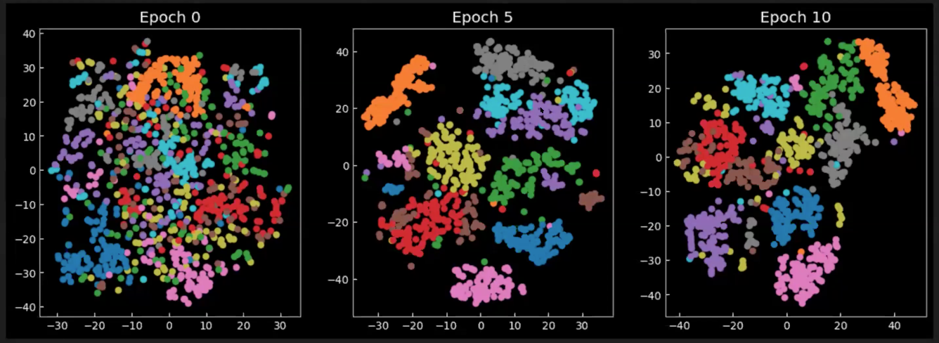
Fig. 8: 2D projection of the means $\E(\vect{z})$ in latent space
📝 Richard Pang, Aja Klevs, Hsin-Rung Chou, Mrinal Jain
24 March 2020